Costa Rica Prototype System Elements
Introduction
The Costa Rica mini project involved producing a prototype website using species data provided in a CSV file. From the time the Costa Rica mini project was announced, we had approximately one week to complete the prototype. For the purpose of the Costa Rica mini project, it wasn’t necessary to vet the occurrence data.
What Needed To Be Done
To produce a prototype that met the client’s requirements, it was necessary to do the following:
-
The input CSV species occurrence data needed to be modified to allow our web application to access it.
-
Distribution ascii grid files needed to be generated for the species.
-
The threshold information for the ascii grids needed to be made available to our web application
-
Our map server installation, and associated map script files, needed to:
- generate coloured raster images using the distribution maps.
- generate legend images for the distribution maps. The legend needed to include the threshold information for the map.
-
The web application needed to provide a single-page interface to allow the user to select a target species.
-
Based on the target species, the web application needed to provide an interactive map showing:
- the species occurrences.
- the species distribution maps.
- the legend of the distribution map.
System Elements
We can break what needed to be done into the following sections:
- Importing
- Modeling
- Mapping
- Web Application
Importing
Normally our importing process involves gathering species occurrence records from ALA. Tom is our resident expert on ALA importing. For more information on our normal ALA importing procedure, read Tom’s post on the ALA import procedure
As the species occurrence data was provided to us in the form of a CSV, the importing process was fairly trivial.
The importing process was performed via a python script that read the contents of the CSV file, and injected the appropriate table data into our SQL database. Tom’s ALA import src code was written in an extensible way that allowed for the Costa Rica specific import code to easily hook into the existing import code base.
The import python script does the following:
-
Wipe the database.
-
Add a source reference for costa rica csv to the sources table.
-
Specify the import time for the source to now.
-
Iterate over each row in the input CSV:
-
Determine if the species is already in our species table.
- If the table doesn’t contain species X: add the species to the table.
-
Add the species occurrence to the occurrences table.
-
Modeling
As part of our main ALA branch, we’ve produced scripts to work with the HPC to generate distribution maps for Australian bird species. These scripts only work for Australian data, as they require existing training data. For this reason, our normal modeling scripts weren’t applicable to the Costa Rica data. Jeremy, our client, produced the distribution maps for the Costa Rica species.
Mapping
Our web interface uses OpenLayers to provide our interactive map. We are using Map Server and the associated PHP library, Map Script, to generate map layer images from the model output ascii grid files.
OpenLayers
OpenLayers is the javascript library we used to provide our interactive map.
How OpenLayers interacts with our PHP Map Script files can be described roughly as follows:
In OpenLayers, we specify our distribution layer as follows:
distribution = new OpenLayers.Layer.WMS(
    "Distribution",
    map_tool_base_url + 'map_with_threshold.php', // path to our map script handler.

    // Params to send as part of request (note: keys will be auto-upcased)
    // I'm typing them in caps so I don't get confused.
    {
        MODE: 'map',
        MAP: 'costa_rica.map',
        DATA: (species_sci_name_cased + '/outputs/' + species_sci_name_cased + '.asc'),
        SPECIESID: species_id,
        REASPECT: "true",
        TRANSPARENT: 'true',
        THRESHOLD: species_distribution_threshold
    },
    {
        // It's an overlay
        isBaseLayer: false,
        transitionEffect: 'resize',
        singleTile: true,
        ratio: 1.5,
    }
);
The above creates an OpenLayers WMS layer.
The params specify our map settings. These will be sent as request paramaters by OpenLayers when it requests the map image for the species. The map paramaters I want to focus on are:
- MAP:
costa_rica.map - DATA:
<species_sci_name_cased>/outputs/<species_sci_name_case>.asc - THRESHOLD:
<species_distribution_threshold>
As well as the paramaters I’ve listed here, OpenLayers will also send paramaters specifying: the WMS version it is using, the projection it is using, the bounding box (BBOX) of the map image it wants, the height and width of the map image (in pixels), etc.
The full list of paramaters supported is available via the OGC (open geo spatial) WMS standard page. You’ll need to download the OpenGIS Web Map Service (WMS) Implementation Specification, and then view section 7.3.2: GetMap request overview.
The MAP paramater defines our map file. I will describe the map file in the Map Server section.
The DATA paramater defines the input data file for our layer. In this case, the ascii grid file for the target species. For the Costa Rica project, the ascii grid files were stored on the map server machine in a predictable location, i.e. knowing the target species name, we could predict where the associated data file would be.
The THRESHOLD paramater is not part of the WMS standard, it is a custom paramater that we used to define the threshold we want to apply to the rendered map. As well as producing ascii grid files, the species distribution models also output a threshold value. Jeremy, our client, asked that the maps not display coloured distribution information for any value below the output threshold. Given the one week deadline for the Costa Rica project, it was decided to store the model output threshold information in our species database. To accomodate this, our import script was modified slightly to also process and store the model output threshold value.
As the user moves the map around, and zooms in and out, OpenLayers makes requests to the map server at the <map_tool_base_url>/map_with_threshold.php URL. The returned image is then overlayed onto the base layer. We provided the option of Google Maps, Bing Maps and Open Street Maps for the base layer. The map_with_threshold.php URL points to our map script php file used to generate map images with input threshold values.
Map Server and Map Script
Map Server does a lot of things. For our purposes, we will use it to generate map images from ascii grid files. We do this by specifying:
-
A map file, which is essentially a config file.
- It is important to keep in mind that the contents of the map file are only defaults, and so can be overwridden by WMS paramaters.
-
A data file, which acts as the data input to generate the map from.
The Map File
The following is our Costa Rica map file:
MAP
PROJECTION
"init=epsg:900913"
END
#define the image type
IMAGETYPE PNG8
#define the area
EXTENT -20037508.34 -20037508.34 20037508.34 20037508.34
UNITS meters
#define the size of output image
SIZE 256 256
#define the working folder of this map file
SHAPEPATH "/scratch/jc155857/CostaRica/models/"
#define the background color
TRANSPARENT ON
IMAGECOLOR 255 255 255
# SCALEBAR object
SCALEBAR
LABEL
COLOR 0 0 0
ANTIALIAS true
SIZE large
END
STATUS ON
END
# LEGEND object
LEGEND
STATUS ON
LABEL
COLOR 0 0 255
END
KEYSIZE 32 16
END
#define the folder that used for generate image
WEB
IMAGEPATH '/www/html/map_script/tmp/'
IMAGEURL 'http://www.hpc.jcu.edu.au/tdh-tools-2:81/map_script/tmp/'
END
#the layer for raster data. you can put multiple layers in one map file
LAYER
NAME "DISTRIBUTION"
TYPE RASTER
STATUS ON
PROCESSING "SCALE=AUTO"
PROJECTION
"init=epsg:4326"
END
#define the transparent of image. 100 is not transpartent.
#0 is totally transparent.
TRANSPARENCY 60
#define the color table. color are define as RGB color from 0 to 255.
#EXPRESSION are used to define the style apply to the right rang of data
#COLORRANGE and DATARANGE are paired to generate gradient color
CLASSITEM "[pixel]"
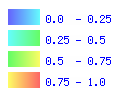
CLASS
NAME "0.0 - 0.25"
KEYIMAGE "ramp_0_25.gif"
EXPRESSION ([pixel]>0 AND [pixel]<0.25)
STYLE
COLORRANGE 0 0 255 0 255 255
DATARANGE 0 0.25
END
END
CLASS
NAME "0.25 - 0.5"
KEYIMAGE "ramp_25_50.gif"
EXPRESSION ([pixel]>=0.25 AND [pixel]<0.5)
STYLE
COLORRANGE 0 255 255 0 255 0
DATARANGE 0.25 0.5
END
END
CLASS
NAME "0.5 - 0.75"
KEYIMAGE "ramp_50_75.gif"
EXPRESSION ([pixel]>=0.5 AND [pixel]<0.75)
STYLE
COLORRANGE 0 255 0 255 255 0
DATARANGE 0.5 0.75
END
END
CLASS
NAME "0.75 - 1.0"
KEYIMAGE "ramp_75_100.gif"
EXPRESSION ([pixel]>=0.75)
STYLE
COLORRANGE 255 255 0 255 0 0
DATARANGE 0.75 1
END
END
END
END
There may appear to be a lot going on in the map file, but once we break it down, you can see that it is actually fairly straight forward.
We specify that we want our map file to be in the projection espg:900913. This is the projection that google maps uses, spherical mercator. This means that all input paramaters to the map file are expected to be in this projection. To be able to define the projection in your map file like this, it needs to be defined in your epsg file. This is described in an OpenLayers spherical mercator doc. The following is what it says to do: add the following line to the base of your epsg file /usr/share/proj/epsg:
<900913> +proj=merc +a=6378137 +b=6378137 +lat_ts=0.0 +lon_0=0.0 +x_0=0.0 +y_0=0 +k=1.0 +units=m +nadgrids=@null +no_defs
We define our output image type to be png.
We define out image extent and measurement units.
We provide a default image size of 256 by 256 pixels.
We provide a SHAPEPATH. All our data file paths will be looked for relative to the SHAPEPATH.
We specify whether or not our image should be transparent, and what colour should be used as the transparent colour marker.
We specify configuration for our SCALEBAR. The scale bar is the bar that shows that 1 cm on your map is X distance on the generated image.
We specify configuration for our Legend.
The KEYSIZE defines the image dimensions of our KEYIMAGE images. The key image is the legend element icon.
We specify our WEB specific options. These include where to write generated map images to, and what the URL is to the image folder.
We define our LAYER. The layer represents our distribution data. A single map file can have multiple layers. In this case, we only have one layer.
The distribution layer’s projection is not spherical mercator, instead, it uses decimal latitude and longitude (epsg:4326).
Normally a data attribute would be specified for a layer. We don’t do this, because we only ever specify the data for the layer via the WMS request paramters.
Where the layer configuration gets interesting is at the attribute CLASSITEM "[pixel]". This is where we define how to interpret the input data and draw the layer. The input ascii grid file describes the distribution likelihood as a value between 0 and 1. 0 represents never will be here, and 1 means definitely should be here. We specify 4 classes for this class item.
- 0 to 0.25
- 0.25 to 0.5
- 0.5 to 0.75
- 0.75 to 1
I’ll explain one of these in detail. From that, the rest should be self explanatory.
CLASS
    NAME "0.0  - 0.25"
    KEYIMAGE "ramp_0_25.gif"
    EXPRESSION ([pixel]>0 AND [pixel]<0.25)
    STYLE
        COLORRANGE  0 0 255 0 255 255
        DATARANGE   0 0.25
    END
END
The name of the class is what will be displayed in the legend.
The expression is a check to see what data to apply this class to.
The style defines how to draw this data. In this case, we use a colour range and an associated data range. The colour selected for this data will depend on where it sits on the data range. This provides a smooth colour transition for the entire data range.
The key image is the image icon to use for the legend. If a key image is not defined, the key icon is generated based on the color defined within the class style. This is where something silly can happen… If instead of a color range (COLORRANGE), a single color (COLOR) is defined, the key image will be a generated icon coloured COLOR of dimensions KEYSIZE. When a COLORRANGE is defined and no key image is defined, the key icon appears to be the last color generated. If no data passes the class’s expression check, then the key icon is empty (no key icon).
The following image shows the map colour transition:
Map Script
Map Script is the php library we use to interface with Map Server.
The following is how a normal map script file interacting with OpenLayers via the WMS standard looks:
    $map_request = ms_newOwsRequestObj();
    $map_request->loadparams();

    $map_path = realpath('./');
    $map_file = null;
    $map_file = $_GET['MAP'];

    $map = ms_newMapObj(realpath($map_path.'/'.$map_file));
    $map->loadOWSParameters($map_request);

    $data = null;
        $data = $_GET['DATA'];

    $layer = $map->getLayerByName('DISTRIBUTION');

    $layer->set('data', $data);

    $map_image = $map->draw();

    // Pass the map image through to view

    header('Content-Type: image/png');
    $map_image->saveImage('');
    exit;
blog comments powered by Disqus
